Regression Analysis
What is Regression Analysis[1]
Regression Analysis is a reliable method of identifying which variables have an impact on a topic of interest. The process of performing a regression allows you to confidently determine which factors matter most, which factors can be ignored, and how these factors influence each other. In order to understand regression analysis fully, it’s essential to comprehend the following terms:
- Dependent Variable: This is the main factor that you’re trying to understand or predict.
- Independent Variables: These are the factors that you hypothesize have an impact on your dependent variable.
Regression analysis is the “go-to method in analytics and smart companies use it to make decisions about all sorts of business issues. Most companies use regression analysis to explain a phenomenon they want to understand (for example, Why did customer service calls drop last month?); predict things about the future (for example, What will sales look like over the next six months?); or to decide what to do (for example, Should we go with this promotion or a different one?).
How Regression Analysis Works[2]
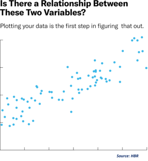
To conduct a regression analysis, you gather the data on the variables in question. (Reminder: You likely don’t have to do this yourself, but it’s helpful for you to understand the process your data analyst colleague uses.) You take all your monthly sales numbers for, say, the past three years and any data on the independent variables you’re interested in. So, in this case, let’s say you find out the average monthly rainfall for the past three years as well. Then you plot all that information on a chart that looks like this:
The y-axis is the number of sales (the dependent variable, the thing you’re interested in, is always on the y-axis), and the x-axis is the total rainfall. Each blue dot represents one month’s data—how much it rained that month and how many sales you made that same month.
Glancing at this data, you probably notice that sales are higher on days when it rains a lot. That’s interesting to know, but by how much? If it rains three inches, do you know how much you’ll sell? What about if it rains four inches?
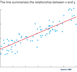
Now imagine drawing a line through the chart above, one that runs roughly through the middle of all the data points. This line will help you answer, with some degree of certainty, how much you typically sell when it rains a certain amount.
This is called the “regression line,” and it’s drawn (using a statistics program like SPSS or STATA or even Excel) to show the line that best fits the data. In other words, explains Redman, “The red line is the best explanation of the relationship between the independent variable and dependent variable.”
In addition to drawing the line, your statistics program also outputs a formula that explains the slope of the line and looks something like this:
y = 200 + 5x + error term
Ignore the error term for now. It refers to the fact that regression isn’t perfectly precise. Just focus on the model:
y = 200 + 5x
This formula is telling you that if there is no x then y = 200. So, historically, when it didn’t rain at all, you made an average of 200 sales and you can expect to do the same going forward, assuming other variables stay the same. And in the past, for every additional inch of rain, you made an average of five more sales. “For every increment that x goes up one, y goes up by five,” says Redman.
Now let’s return to the error term. You might be tempted to say that rain has a big impact on sales if for every inch you get five more sales, but whether this variable is worth your attention will depend on the error term. A regression line always has an error term because, in real life, independent variables are never perfect predictors of the dependent variables. Rather the line is an estimate based on the available data. So, the error term tells you how certain you can be about the formula. The larger it is, the less certain the regression line.
The above example uses only one variable to predict the factor of interest — in this case, rain to predict sales. Typically you start a regression analysis wanting to understand the impact of several independent variables. You might include not just rain but also data about a competitor’s promotion. “You keep doing this until the error term is very small,” says Redman. “You’re trying to get the line that fits best with your data.” Although there can be dangers in trying to include too many variables in a regression analysis, skilled analysts can minimize those risks. And considering the impact of multiple variables at once is one of the biggest advantages of regression analysis.
Regression Analysis in Finance[3]
Regression analysis comes with several applications in finance. For example, the statistical method is fundamental to the Capital Asset Pricing Model (CAPM). Essentially, the CAPM equation is a model that determines the relationship between the expected return of an asset and the market risk premium.
The analysis is also used to forecast the returns of securities, based on different factors, or to forecast the performance of a business.
- Beta and CAPM: In finance, regression analysis is used to calculate the Beta (volatility of returns relative to the overall market) for a stock. It can be done in Excel using the Slope function.
- Forecasting Revenues and Expenses: When forecasting financial statements for a company, it may be useful to do a multiple regression analysis to determine how changes in certain assumptions or drivers of the business will impact revenue or expenses in the future. For example, there may be a very high correlation between the number of salespeople employed by a company, the number of stores they operate, and the revenue the business generates.
Excel remains a popular tool to conduct basic regression analysis in finance, however, there are many more advanced statistical tools that can be used. Python and R are both powerful coding languages that have become popular for all types of financial modeling, including regression. These techniques form a core part of data science and machine learning where models are trained to detect these relationships in data.
Types of Regression Analysis[4]
There are two types of regression analysis: single-variable linear regression and multiple regression.
Single-variable linear regression is used to determine the relationship between two variables: the independent and dependent. The equation for a single variable linear regression looks like this:
ŷ=α+βx+ε
In the equation:
ŷ is the expected value of Y (the dependent variable) for a given value of X (the independent variable).
x is the independent variable.
α is the Y-intercept, the point at which the regression line intersects with the vertical axis.
β is the slope of the regression line, or the average change in the dependent variable as the independent variable increases by one.
ε is the error term, equal to Y – ŷ, or the difference between the actual value of the dependent variable and its expected value.
Multiple regression, on the other hand, is used to determine the relationship between three or more variables: the dependent variable and at least two independent variables. The multiple regression equation looks complex but is similar to the single variable linear regression equation:
ŷ=α+β1x1+β2x2+...βkxk+ε
Each component of this equation represents the same thing as in the previous equation, with the addition of the subscript k, which is the total number of independent variables being examined. For each independent variable you include in the regression, multiply the slope of the regression line by the value of the independent variable, and add it to the rest of the equation.
History of Regression Analysis[5]
The earliest form of regression was the method of least squares, which was published by Legendre in 1805, and by Gauss in 1809. Legendre and Gauss both applied the method to the problem of determining, from astronomical observations, the orbits of bodies about the Sun (mostly comets, but also later the then newly discovered minor planets). Gauss published a further development of the theory of least squares in 1821, including a version of the Gauss–Markov theorem.
The term "regression" was coined by Francis Galton in the 19th century to describe a biological phenomenon. The phenomenon was that the heights of descendants of tall ancestors tend to regress down towards a normal average (a phenomenon also known as regression toward the mean). For Galton, regression had only this biological meaning, but his work was later extended by Udny Yule and Karl Pearson to a more general statistical context. In the work of Yule and Pearson, the joint distribution of the response and explanatory variables is assumed to be Gaussian. This assumption was weakened by R.A. Fisher in his works of 1922 and 1925. Fisher assumed that the conditional distribution of the response variable is Gaussian, but the joint distribution need not be. In this respect, Fisher's assumption is closer to Gauss's formulation of 1821.
In the 1950s and 1960s, economists used electromechanical desk "calculators" to calculate regressions. Before 1970, it sometimes took up to 24 hours to receive the result from one regression.
Regression methods continue to be an area of active research. In recent decades, new methods have been developed for robust regression, regression involving correlated responses such as time series and growth curves, and regression in which the predictor (independent variable) or response variables are curves, images, graphs, or other complex data objects, regression methods accommodating various types of missing data, nonparametric regression, Bayesian methods for regression, regression in which the predictor variables are measured with error, regression with more predictor variables than observations, and causal inference with regression.
See Also
References


